9.7 Vectors

Mathematically, a vector is a value consisting of a magnitude and a direction^[1]. It is interpreted geometrically as an arrow drawn from one point to another. This interpretation implies a location for the vector, but location is not an intrinsic property of vectors. To remove location from the discussion, the beginning of the arrow is assumed to be located at some given origin. A vector with an assumed origin is called a position vector.

In Myron, composite values are used to represent points. It does not matter which of the composite types are used: radial, vector or complex^[2]. The radial type represents the angle-magnitude form of a point and the vector type represents the coordinate form of a point. A complex value, being a composite type, represents a point in two-space. Operations appropriate for each composite type are provided as well as methods to convert between them.

In the discussion that follows, the terms vector and position vector are used in the mathematical sense and the terms vector and radial when used together with the qualifiers type and value refer to Myron types and values.

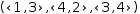
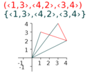
The plotter provides graphical representations of line segments and position vectors by interpreting adjacent Myron vectors in a tuple as line segments and Myron vectors in a set as position vectors. Thus ((1, 3)ʋ, (4, 2)ʋ, (3, 4)ʋ) is two line segments and {(1, 3)ʋ, (4, 2)ʋ, (3, 4)ʋ} is three position vectors. Figure 9.13 shows the plot of these collections.

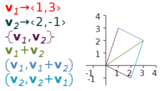
Addition and subtraction of vectors also has a geometric interpretation. The sum of the vectors v_1ʋ→(1, 3)ʋ and v_2ʋ→(2, -1)ʋ is given simply by v_1ʋ+v_2ʋ. v_2ʋ can be translated into a line segment whose origin is at v_1ʋ by (v_1ʋ, v_1ʋ+v_2ʋ). Similarly, v_1ʋ can be translated by (v_2ʋ, v_2ʋ+v_1ʋ). Plotting all these expressions yields the usual vector-addition parallelogram in Figure 9.14.

The simplicity of the vector expressions above belies behind-the scenes details.

9.7.1 Vector Addition

Vector addition falls into three cases: adding (or subtracting) two vectors, adding a vector and a scalar and adding one type of vector onto another. The latter case is described in §9.7.4.

Addition and subtraction between two vector values are straightforward applications of the rules for tuples with matching common types: corresponding elements of a vector are added. Addition and subtraction between two radial values uses conversion to and from intermediate vector values. This means that addition of the innocuous looking (1, ℼ/4)ɽ+(2, ℼ/6)ɽ leads to

This simplifies to but evaluates to the simpler (2.977197223086887, 0.6106424421303817)ɽ (with more sub tabula precision than the three digits shown).

9.7.2 Scalar Multiplication

Scalar multiplication of a vector has the effect of changing (scaling) the vector's length.

Multiplication of a line segment by a scalar changes both ends of the line segment. α⋅(v_1ʋ, v_2ʋ) is (α⋅v_1ʋ, α⋅v_2ʋ). To scale just the length of a line segment whose origin is not at zero, the line segment has to be translated to the origin, scaled and translated back. That is, given vectors v_1ʋ→(1, 3)ʋ, v_2ʋ→(2, -1)ʋ and line segment lsʈ→(v_1ʋ, v_2ʋ), the expression (lsʈ-v_1ʋ)⋅2+v_1ʋ is a line segment with origin v_1ʋ that has the same direction and twice the length of lsʈ. This can be seen by performing substitutions and simplification.

Using the radial type, a magnitude-angle pair is represented directly by (m, θ)ɽ. Multiplication by a scalar is straightforward: 2⋅(m, θ)ɽ is (2⋅m, θ)ɽ.

9.7.3 Vector Multiplication

Multiplying two vectors produces a scalar using a dot-product operation. Syntactically, dot product is inferred for the multiplication operator when the left operand is a row vector and the right operand is a column vector. Thus

produces v_1⋅w_1+v_2⋅w_2+v_3⋅w_3. Note the similarity of display between this and multiplication between a row matrix and a column matrix. [(v_1, v_2, v_3)]×[(, w_1), (, w_2), (, w_3)] produces [(, v_1⋅w_1+v_2⋅w_2+v_3⋅w_3)]. However, vector multiplication always produces a scalar whereas matrix multiplication always produces a matrix, albeit a unit matrix in this case.

Vector multiplication is not defined for other combinations of vectors. Expressions with mixed operands are caught by the parser when the type of the result is important. If mixed vectors are required by some mathematical context, explicit casts can be used to specify conversions that conform to Myron's rules for vector multiplication.

Dot product should not be confused with the residual rule for tuples. The tuple versions of the expressions above are (v_1, v_2, v_3)⋅(w_1, w_2, w_3) and (v_1⋅w_1, v_2⋅w_2, v_3⋅w_3).

Applied to radial values, dot product uses an intermediate conversion to vector values. (m_1, θ_1)ɽ∘(m_2, θ_2)ɽ produces the scalar value (after simplification)

.

9.7.4 Mixing Vector Types

When a composite value is mixed with an operand of another type under addition or subtraction, the type of the result is the “highest” type of either operand according to the ordering radial, column, row, matrix. The operand not of the highest type is converted to the highest type before the operation is applied. Thus (m, θ)ɽ+(a, b)ʋ produces (m⋅cos θ+a, m⋅sin θ+b)ʋ Forcing the row vector to a radial (m, θ)ɽ+(a, b)ʋɽ produces

(√((a+m⋅cos θ)^2+(b+m⋅sin θ)^2), arctan ((b+m⋅sin θ)÷(a+m⋅cos θ)))ɽ.

 

If mixing composite types leads to uncertainty as to which automatic conversions are applied, explicit casts can be used to remove the uncertainty.

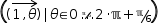
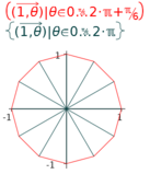
9.7.5 Vector Example

To exercise Myron's approach to vectors, consider the problem of drawing 12 vectors each leading from the centre of a clock to the numbers on its face. The vectors can be generated by the expression {(1, θ)ɽ|θ∈0, 2⋅ℼ, ℼ/6}. The generator produces a set of 12 vectors. The use of sets causes the vectors to be plotted as position vectors. Contrast this with ((1, θ)ɽ|θ∈0, 2⋅ℼ+ℼ/6, ℼ/6) which produces a tuple of 13 vectors. When plotted, the use of tuples causes the position vectors to be treated as points and draws them as 12 continuous line segments. The results are shown in Figure 9.15.